Purdue Wildlife Area: Data Collection, Processing, and Analysis (AT319 Final Project)

 

 

 

 

 

 

 

 

 

 

Purdue Wildlife Area: Data Collection,

Processing, and Analysis

 

Kendrick Wittmer

AT 31900

Dr. Joseph Hupy

May 5, 2025

 

 

 

 

 

 

 

 

 

 

 

Introduction

            The ability to collect data, process it, and perform further analysis in a Geographic Information System (GIS) is a fundamental skill in the UAS industry. Simple aerial images without further processing only provide so much information. Instruction on various forms of analysis has been provided throughout the course of AT 319. The objective of this project is to execute a mapping mission in an assigned area at the Purdue Wildlife Area (PWA) and to engage in a variety of post processing analyses using ArcGIS Pro in order to demonstrate proficiency in GIS analysis.

Data Collection

            As previously mentioned, the predetermined area of study was the PWA, particularly zone 9 (figure 1). My partner (Mason Santana) and I decided the appropriate platform and sensor for this application would be the DJI Matrice 300 RTK equipped with the Zenmuse P1. The real time kinematic (RTK) GPS correction allows for accurate geolocation of images while minimizing time spent correcting images in the pre-processing phase. The survey area consisted primarily of a pond and wooded area in the northernmost portion of the PWA, allowing us to utilize a small gravel lot located at a dock as a takeoff point (figure 2). The flight was conducted in around 45 total minutes with only minor complications due to high wind which necessitated a battery swap (figure 3). The flight was conducted at an altitude of 122 meters and overlap and sidelap were set to 80% and 85% respectively. Upon successful completion of the flight, data collected was transferred from the sensor SD card to an SSD to transport the images.

Figure 1: Mission Area Assignments

 

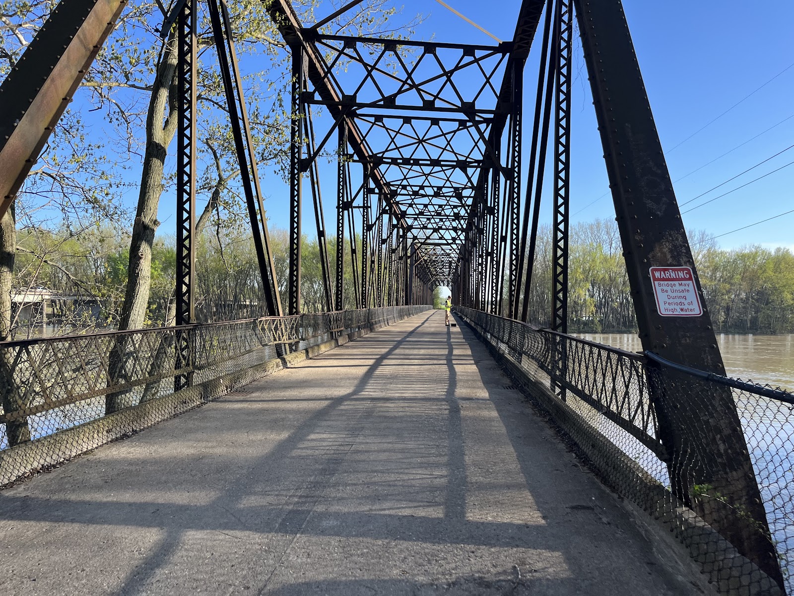
Figure 2: Takeoff Point

 

 

 

 

 

General
Location	Purdue Wildlife Area
Date	4/14/2024
Vehicle	DJI Matrice 300
Sensor	Zenmuse P1
Flight Information
Flight Number	1
Takeoff Time	2:45pm
Landing Time	3:15pm
Altitude (m)	122m
Sensor Angle	Nadir
Overlap	80%
Sidelap	85%
Flight Number	2
Takeoff Time	3:20pm
Landing Time	3:35pm
Altitude (m)	122m
Sensor Angle	Nadir
Overlap	80%
Sidelap	85%
Images Collected	1,268
File Size	20.1GB
Storage Location (SSD)	"D:\AT319\Final Project\Data\DCIM"
Ground Control
System Used	RTK
Coordinate System	WGS 1984
Weather
Cloud Cover	Overcast
Wind Direction	West
Wind Speed	20mph
Temp	65 degrees Fahrenheit
Crew
PIC	Mason Santana
VO	Kendrick Wittmer

Figure 3: Flight Metadata

 

 

Processing

            Immediately following the flight, the data was transferred to the temp folder of PC06 in NISW 145 for processing in ArcGIS Drone2Map (figure 4,16). Minimal changes to settings were required due to the use of RTK correction. Only the desired 2D and 3D products had to be selected, which were orthomosaic, DSM, and shaded DSM. The exact processing time is unknown as it was set to run overnight, however due to the large number of images in the dataset it is safe to assume it took several hours or more.

PC#	06
File location	C:\temp\mtsantan\Data\DCIM
Images	1268

Figure 4: Raw Data Processing Location

 

2D and 3D Products

            The number of images collected with the P1 and processing time was reflected in the quality of the outputs. The orthomosaic was produced with such high quality that you could zoom in and see individual downed trees and trails/paths could be easily distinguished (figure 5). The digital surface model was also of remarkable quality, except for some spots of minor distortion upon the surface of the water due to excessive wind throughout the flight (figure 6). The shaded DSM was created by applying an appropriate color ramp to the DSM and overlaying the generated hillshade at 33% transparency, creating a map which allows for easy interpretation of the survey area’s changes in elevation and surface features. Figure 8 highlights the differences between each product with the orthomosaic providing a clear image of colors and what types of terrain are present and the DSM highlighting the changes in terrain.

Figure 5: Mission Orthomosaic

Figure 6: Shaded DSM

Figure 7: Shaded DSM vs. Orthomosaic Comparison

Digitizing

            The skill of digitizing in GIS analysis allows the creator to present data to the reader in an easy-to-understand way and can be used to gather data such as length, area, and volume within a digitized area. The first digitized map for this project involves the roads at the PWA. While different types of roads were specified, all roads were digitized under one polyline feature class (figure 8). A new domain was added which allows the type of road to be specified in a field titled “Roads” that was also added (figure 18).

 

Figure 8: Digitized Roads

 

            The other requested product was a digitized map of the landcover at the PWA. The process for digitizing landcover was the same as the roads being that it was done under 1 feature class with different domains. The main difference is that landcover was digitized with polygons, not lines. Additionally, I restricted the landcover digitization to the assigned boundary for the flight in order to create clean edges which the polygons could snap to. 

Figure 9: Digitized Landcover

Classification

            Two types of classification analyses were performed for this project: unsupervised and supervised. Prior to conducting any classification, the raw orthomosaic was first resampled to a larger cell size of 0.5 using a bilinear sampling technique (figure 19). Increasing the cell size decreases the number of pixels in the image which simplifies the classification process and reduces processing times.

            The process for running unsupervised classification was simple. The resampled orthomosaic was used as the input along with the default schema, which was later edited to include the desired classes of trees, water, roads, and fields. Spectral detail was set to 15.50, spatial detail to 15, and minimum segment size to 100 (figure 20)

            The following settings were used for training settings (figure 21). While the desired number of classes was 4, when the maximum number of classes was set to 4 only 3 were produced.

            The initial unsupervised product will be difficult to interpret as the symbology for the segments will be switched around. Unfortunately, even after appropriately coloring the classes, the unsupervised classification did not turn out particularly great (figure 10). The pond and roads have well defined boundaries; however, it appears to have classified most of the forest area as water. This is a problem we can address when doing supervised classification in which training samples specify what type of landcover is in each area of the image.

Figure 10: Unsupervised Classification

               The process for supervised classification involved the same basic settings, however it does include the additional step of creating training classes to help define areas of landcover (figure 11). One pattern that became apparent after several attempts at supervised classification was a few quality samples produce much better results than many samples which were selected with less care. A few good samples that capture which color pixels are associated with each type of landcover are all that is required. The final product of this classification showed clearly defined areas of water, roads, and more impressively differentiated the trees from fields (figure 12).

Figure 11: Supervised Classification Training Samples

Figure 12: Supervised Classification

 

Raster Analysis

            Performing raster analysis in ArcGIS allows the user to dig deeper than what is visually apparent in a data set and look for more specific patterns. The required product for this portion is a reclassed DSM showing objects higher than 6 meters. Through use of the raster calculator with the DSM as the input, a simple greater than formula can be used for this (figure 22). To determine a base height to add 6 meters to, I simply clicked on several flat surfaces throughout the DSM which demonstrated an average base height of 213. All objects at a height greater than 6 meters are assigned a value of 1 and the rest 0. Through the symbology settings, the 0 values were then set to transparent and 1 as red, and the reclassed DSM was overlayed on the orthomosaic (figure 13).

Figure 13: Reclassed DSM

            The next product to be created was a 10-meter buffer along two track roads. First, I created a new copy of the roads feature class and deleted the other non-Two Track roads. The process of creating a buffer was simple. The new roads feature class was inputted into the buffer tool and the distance was set to 10 meters, creating a 10-meter buffer on either side of the road.

Figure 14: Two-Track Road Buffer

            This 10m buffer created using the buffer tool is a form of vector data, saved as a feature class. In order to perform further analysis, we must convert this to a raster using the Polygon to Raster tool. This tool is relatively simple to use, first input the feature class, then select whatever field designates this class as the value field. In this case it was “roads” with a value of 4 (figure 24). This will then generate a raster of the polygon area.

Figure 15: Raster Buffer of Two-Track Roads

            The final data product to be produced involves using the data from the previous three maps to identify trees which are located within 10 meters of roads. The Raster Calculator tool is utilized to accomplish this with a conditional formula which assigns a value of 1 to all areas covered by the reclassed DSM and raster buffer (figure 25). The result is a raster which shows all objects 6 meters or higher off the ground (trees) within 10 meters of the road, which when overlayed over the orthomosaic provides a clear image of where these trees are located (figure 16). This may be useful to a landowner as this indicates areas with large trees near roadways. A landowner may want to cut down or trim some of these trees as they may pose a hazard by blocking the road if the tree were to fall or drop limbs.

Figure 16: Trees Near Roads

Conclusion

        From data collection to processing and analysis, this project served as an opportunity to demonstrate the various skills in ArcGIS acquired throughout the past semester and has allowed me to further understand the vast capabilities of GIS. The data products created within this assignment culminate nearly everything we have learned and are evidence of at least a basic level of proficiency in ArcGIS Pro. Many employment opportunities within the UAS industry, whether with a business or through independent contracting, are based on GIS operations. Moreover, continuing to improve on these skills will help me form a strong foundation for which a career in UAS can be built on.

Appendix

Figure 17: Imported Mission in Drone2Map

Figure 18: Road Digitization Attribute Table

Figure 19: Ortho Resampling Settings

Figure 20: Segmentation Settings

Figure 21: Training Settings

Figure 22: Reclassed DSM Formula

Figure 23: Buffer Settings

Figure 24: Polygon to Raster Settings

Figure 25: Raster Calculator Settings for 6m Trees within 10m Buffer

ArcGIS Pro Project File Location (PC04)

C:\temp\kwittme\Wittmer_AT319_FinalProject.aprx

Figure 26: Project File Location